From a ZIP code to a living tree map.
I used ZIP code 07042 in New Jersey as the starting point for turning aerial and satellite imagery into georeferenced results. The project locates tree candidates, studies canopy seasonality and combines that signal with daily weather to estimate how leaf load changes throughout autumn.
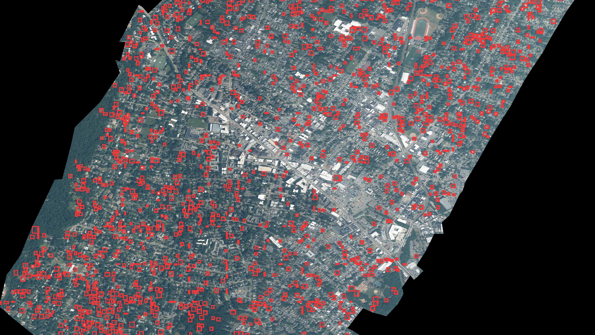
One territorial query turned into four usable outputs.
The analysis produced an annotated image for visual inspection, a GeoJSON of georeferenced boxes, a coordinate CSV and a run summary. From 4,312 initial proposals, the filter retained 1,986 candidates with sufficient vegetation signal and removed 2,326 detections during quality control.
Preserve the geography after inferring in pixels.
Acquire the raster
The pipeline works with a NAIP mosaic at approximately 0.87 meters per pixel for the area defined by ZIP code 07042.
Detect by tiles
DeepForest processes 800-pixel patches with 25% overlap to reduce losses when a crown crosses an edge.
Transform coordinates
Rasterio converts xmin, ymin, xmax and ymax from pixels into the GeoTIFF CRS. GeoPandas reprojects the result to WGS84.
Export and inspect
The prototype writes a GeoJSON of boxes, a coordinate CSV and an image with every result drawn over the territory.
Detection is only the first layer of the analysis.
The first challenge was making a crown detector work with a large urban raster without losing geographic position. The 4,733 × 5,312-pixel mosaic is divided into 800-pixel tiles with 25% overlap. That overlap prevents a crown from disappearing because it falls exactly across the edge of two windows. Repeated boxes are then consolidated before returning to the file’s coordinate system.
The NAIP image has four bands. Along with RGB, its near-infrared band makes it possible to calculate NDVI and add independent vegetation evidence. Every proposal receives model confidence, median and 75th-percentile NDVI, the fraction of vegetation pixels and the fraction of valid data. Explicit thresholds retain the most consistent detections and record why each one was rejected. In 07042, that quality-control step reduced 4,312 proposals to 1,986 candidates supported by vegetation signal.
The output does not end with a visual. The GeoTIFF affine transform takes every box from pixels into real coordinates; GeoPandas converts it into geometry and reprojects it to WGS84. The same detection can therefore be viewed over the photograph, opened in QGIS, joined to streets or parcels and exported as GeoJSON or CSV.
A small tool with separated responsibilities.
DeepForest as a starting point
The script integrates weecology/deepforest-tree to bring a specialized detector into a custom geospatial pipeline.
Georeference preserved
The transform is read from the input file so every box returns to geographic space instead of remaining trapped in image coordinates.
Interoperable GeoJSON
Boxes are saved as polygons with a score and normalized CRS, ready to explore and review in QGIS.
Annotated image
OpenCV draws rectangles and confidence scores over the raster to quickly review how the detector responded.
Block-based work
Tiling divides large rasters into manageable units and opens a direct route toward GPU processing.
From a detection to a map
The output combines location, geometry and confidence so each object can be filtered, visualized and connected to other territorial data.
Move from “where are the trees?” to “how does their canopy change during the year?”
The second part of the project compares observations from different moments. For a ZIP-code query, the system gets the geographic boundary from Census TIGERweb, uses ESA WorldCover as an initial tree mask and searches for low-cloud Sentinel-2 L2A scenes. In the Northern Hemisphere it takes a leaf-off window from January through March, a leaf-on window from July through August and a third observation close to the chosen date.
The seasonal NDVI difference helps separate signals consistent with deciduous and evergreen vegetation. Where LiDAR is available, canopy height, return penetration and crown shape add another perspective. In the detailed New Jersey run, twelve LiDAR files covered 98.6% of the area and produced 20,987 provisional crowns: 2,930 leaned deciduous, 2,929 leaned evergreen and 15,128 remained in the middle. Keeping that middle category lets the map express the actual strength of the evidence.
Summer as reference
July and August scenes show peak vegetation vigor and establish the canopy signal when leaves are present.
Winter as contrast
January-to-March scenes reveal how much of that signal remains and how much changes with the season.
A query situated in time
The third window connects the seasonal pattern to the day being analyzed instead of returning a static classification.
The calendar provides context; daily weather moves the simulation.
The model moves through every day from the start of the autumn season to the selected date. Day length and accumulated cold control senescence; mean and minimum temperature, humidity and precipitation over the previous fourteen days change stress; wind, gusts, rain and frost affect detachment. Meteorological wind direction is converted to estimate where material travels after leaving the canopy.
Within every 100-meter cell, the system tracks five states: attached green canopy, attached senescent canopy, new fall, load currently on the ground and material removed, degraded or transported outside the area. The user can select ZIP code, date, cell size and a cleanup half-life. Daily data comes from Open-Meteo and is cached so the same request can be repeated without downloading everything again.
For 07042 on November 15, 2025, the historical run began on August 1. The index found both the largest fall pulse and the highest estimated ground load on October 13. That day the season had accumulated 47.9% of its fall and reached a spatial equivalent of 1.42 million m²; by November 15, cumulative fall reached 97.2% and the load still present had dropped to about 554,000 m² through cleanup, dispersion and degradation.
Turn environmental context into a signal for planning and creative work.
Because the output is organized by place and date, it can feed communication decisions that depend on the surrounding environment. A gardening, tools, outdoor cleaning, insurance, mobility or home-services brand could identify the areas and weeks where leaf fall is most relevant, adapt its message to that moment and coordinate media with observable conditions.
Prioritize markets by signal
ZIP codes can be compared by tree-covered area, deciduous component and seasonal progression to decide where a campaign has the strongest context.
Choose the creative moment
The daily series can align cleaning, maintenance, garden or driving messages with the rise, peak and decline of ground leaf load.
Translate data into local creative
The season’s state can feed city-level variants: anticipation before the peak, response during the fall and maintenance afterward.
Understand physical context
Joining cells with streets, parcels or advertising locations can add environmental context to placement selection.
Compare hypotheses
Historical outputs make it possible to study whether weather, seasonality and commercial response move together across markets.
Plan resources
The same map can also prioritize inspections, urban maintenance or service routes before turning that insight into communication.
A system that can be queried, repeated and expanded.
- ZIP-code interface: a query receives location, date, grid size and cleanup rate, then returns a map, timeline, weather and downloads.
- Two levels of detail: NAIP and LiDAR support individual-crown work where available; Sentinel-2 and WorldCover enable a territorial view for new ZIP codes.
- Historical replay: stored weather makes it possible to revisit a date and understand which factors drove the daily change.
- Interoperable outputs: results travel as image, CSV, GeoJSON, GeoTIFF and JSON for integration with maps, dashboards or later analysis.
- Extensible architecture: data sources, the fall model and the presentation layer are separated so one part can evolve without rebuilding the rest.